import networkx as nx

G = nx.DiGraph()
G.add_weighted_edges_from({
    ("A", "B", 20), ("A", "C", 42), ("B", "A", 20),
    ("B", "C", 30), ("C", "A", 42),("C", "B", 30)
})

nx.draw(G)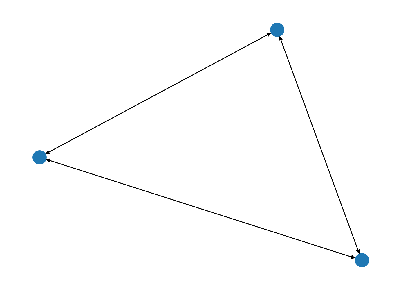
We already saw how we can implement a simple version of the TSP problem.
We will check a simplified version of this problem with just three nodes.
import networkx as nx
G = nx.DiGraph()
G.add_weighted_edges_from({
("A", "B", 20), ("A", "C", 42), ("B", "A", 20),
("B", "C", 30), ("C", "A", 42),("C", "B", 30)
})
nx.draw(G)
So that our final QUBO is represented as…
from collections import defaultdict

lagrange = 120

# Creating the QUBO
Q = defaultdict(float)

# number of steps
N = G.number_of_nodes()

# Objective that minimizes distance
for u, v in G.edges:
    for pos in range(N):
        nextpos = (pos + 1) % N

        # going from u -> v
        try:
            value = G[u][v]["weight"]
        except KeyError:
            value = lagrange # Non existent route cost

        Q[((u, pos), (v, nextpos))] += value

        # going from v -> u
        try:
            value = G[v][u]["weight"]
        except KeyError:
            value = lagrange # Non existent route cost

        Q[((v, pos), (u, nextpos))] += value

# Constraint that each row has exactly one 1
for node in G:
    for pos_1 in range(N):
        Q[((node, pos_1), (node, pos_1))] -= lagrange
        for pos_2 in range(pos_1+1, N): # Next positions
            Q[((node, pos_1), (node, pos_2))] += lagrange

# Constraint that each col has exactly one 1
for pos in range(N):
    for node_1 in G:
        Q[((node_1, pos), (node_1, pos))] -= lagrange
        for node_2 in set(G)-{node_1}:
Q[((node_1, pos), (node_2, pos))] += lagrange # Cost of being in more than one placeNot always available, in particular if we scale up the number of nodes, time-steps and traveling people but a good way to check how good our proposed algorithms are solving it.
import dimod

sampler = dimod.ExactSolver()

response = sampler.sample_qubo(Q)
print(response.slice(0, 15))
('A', 0) ('A', 1) ('A', 2) ('B', 0) ('B', 1) ... ('C', 2) energy num_oc.
0 1 0 0 0 0 ... 0 -536.0 1
1 0 0 1 1 0 ... 0 -536.0 1
2 0 0 1 0 1 ... 0 -536.0 1
3 0 1 0 0 0 ... 0 -536.0 1
4 1 0 0 0 1 ... 1 -536.0 1
5 0 1 0 1 0 ... 1 -536.0 1
6 1 0 0 0 1 ... 0 -520.0 1
7 0 0 1 1 1 ... 0 -520.0 1
8 1 1 0 0 0 ... 0 -520.0 1
9 0 1 0 1 0 ... 0 -520.0 1
10 0 1 1 1 0 ... 0 -520.0 1
11 1 0 1 0 1 ... 0 -520.0 1
12 0 0 0 0 1 ... 0 -480.0 1
13 0 0 0 0 1 ... 1 -480.0 1
14 0 0 0 1 0 ... 1 -480.0 1
['BINARY', 15 rows, 15 samples, 9 variables]route = response.first.sample
cycle = [None]*(N+1)
for key in route:
if route[key] == 1:
cycle[key[1]] = key[0]
cycle[-1] = cycle[0]
cost = sum(G[n][nbr]["weight"] for n, nbr in nx.utils.pairwise(cycle))
print(f"Cost for route {cycle} is {cost}")Cost for route ['A', 'C', 'B', 'A'] is 92from networkx.algorithms import approximation as approx
cycle = approx.simulated_annealing_tsp(G, "greedy", source="A")
cost = sum(G[n][nbr]["weight"] for n, nbr in nx.utils.pairwise(cycle))
print(f"Cost for route {cycle} is {cost}")Cost for route ['A', 'B', 'C', 'A'] is 92For a proper quantum annealing example we would need to use a device like the ones in appendix B. We can do a simplification simulating it locally… First, a conversion to Ising coefficients is needed. Dimod offers many convenient functions to convert between analogous representations.
from quantagonia import HybridSolver, HybridSolverParameters
from quantagonia.qubo import QuboModel

# Qubo to Binary Quadratic Problem
bqm = dimod.BinaryQuadraticModel.from_qubo(Q)

# read bqm file into QuboModel
qubo = QuboModel.from_dwave_bqm(bqm)

# solve QUBO with Quantagonia's solver
API_KEY = os.environ["QUANTAGONIA_API_KEY"]
params = HybridSolverParameters()
hybrid_solver = HybridSolver(API_KEY)
qubo.solve(hybrid_solver, params)
Ising is commonly used for pure quantum approaches.
bqm = dimod.BinaryQuadraticModel.from_qubo(Q)
h, J, offset = bqm.to_ising()
If we follow the instructions in Quantagonia’s documentation we can see it offers a seamless integration with Qiskit and DWave’s modelling libraries. We could also get the pure data out of the dictionaries with named variables so that it gets easier to manage using indexes for the qubits.
# Get the variable names
indexes = list(h.keys())

hp = []
jp = {}
for i in range(len(h)):
    name_i = indexes[i]
    hp += [h[name_i]]
    for j in range(len(h)):
        name_j = indexes[j]
        if (name_i,name_j) in J:
            jp[(i,j)] = J[(name_i,name_j)]
For this simple problem we could follow the approach to a local simulation of the problem implementing the canonical evolution described before. The issue might be managing the problem size that renders a \(2^N \times 2^N\) matrix.
import numpy as np

# Pauli matrices
sigma_x = np.array([[0, 1], [1, 0]], dtype=complex)
sigma_z = np.array([[1, 0], [0, -1]], dtype=complex)
I = np.eye(2, dtype=complex)

def kron_product(matrices):
    """Compute Kronecker product of a list of matrices."""
    result = matrices[0]
    for mat in matrices[1:]:
        result = np.kron(result, mat)
    return result

def transverse_field(N, h=1.0):
    """
    Construct the transverse field term: -h * sum_i sigma^x_i
    """
    dim = 2**N
    H_x = np.zeros((dim, dim), dtype=complex)

    for i in range(N):
        # Build sigma^x_i = I ⊗ ... ⊗ sigma_x (at position i) ⊗ ... ⊗ I
        ops = [I] * N
        ops[i] = sigma_x
        H_x += kron_product(ops)

    return -h * H_x

def problem_hamiltonian(N, h_array, J_matrix):
    """
    Construct the problem hamiltonian hZ + JZZ
    """
    dim = 2**N
    H = np.zeros((dim, dim), dtype=complex)

    for i in range(N):
        # Build sigma^x_i = I ⊗ ... ⊗ sigma_x (at position i) ⊗ ... ⊗ I
        ops = [I] * N
        ops[i] = sigma_z
        H += h_array[i] * kron_product(ops)

    for keys in J_matrix:
        # Build sigma^z_i sigma^z_j
        ops = [I] * N
        ops[keys[0]] = sigma_z
        ops[keys[1]] = sigma_z
        H += J_matrix[keys] * kron_product(ops)

    return H

size = len(h)
H_init = transverse_field(size)
H_problem = problem_hamiltonian(size, hp, jp)
We could check if the solution ot our problem matches the expected one.
import numpy as np
from math import sqrt
from numpy.linalg import eig

def get_gs(h_mat):
    """ Computes the ground state """
    evals, evecs = eig(h_mat)
    sort_index = np.argsort(evals)

    stat_gs = evecs[:, sort_index[0]]
    gs_val = evals[sort_index[0]]

    num = 1
    for idx in sort_index[1:]:
        if evals[idx] == gs_val:
            stat_gs += evecs[:, idx]
            num += 1
        else:
            break

    return np.dot((1/sqrt(num)), stat_gs)

r = np.nonzero(get_gs(H_problem))[0]
print(f"Potential solutions {r}")
Potential solutions [126 235 373 414 435 461]We would need to extract the binary representation of this integer to understand the variables being selected for our solution, but having six values would represent a degenerated basis state with six optimal solutions. We could then perform the state evolution as we did before to get that state from an initial state evolution and see what velocity of mixing Hamiltonians works best.
import matplotlib.pyplot as plt

def get_eigenspectra(h_mat):
    """
    Computes the eigenspectra
    """
    evals, evecs = eig(h_mat)
    sort_index = np.argsort(evals)

    return evals [sort_index], evecs[:, sort_index]

e0 = []
e1 = []
time_range = np.arange(0.0, 1.0, 0.1)

for lambda_t in time_range:

    H = (1-lambda_t)*H_init + lambda_t*H_problem

    vals, stats = get_eigenspectra(H)
    e0.append(vals[0])
    e1.append(vals[1])

plt.plot(time_range, e0, label="$E_0$")
plt.plot(time_range, e1, label="$E_1$")
plt.legend(loc="upper left")
plt.show()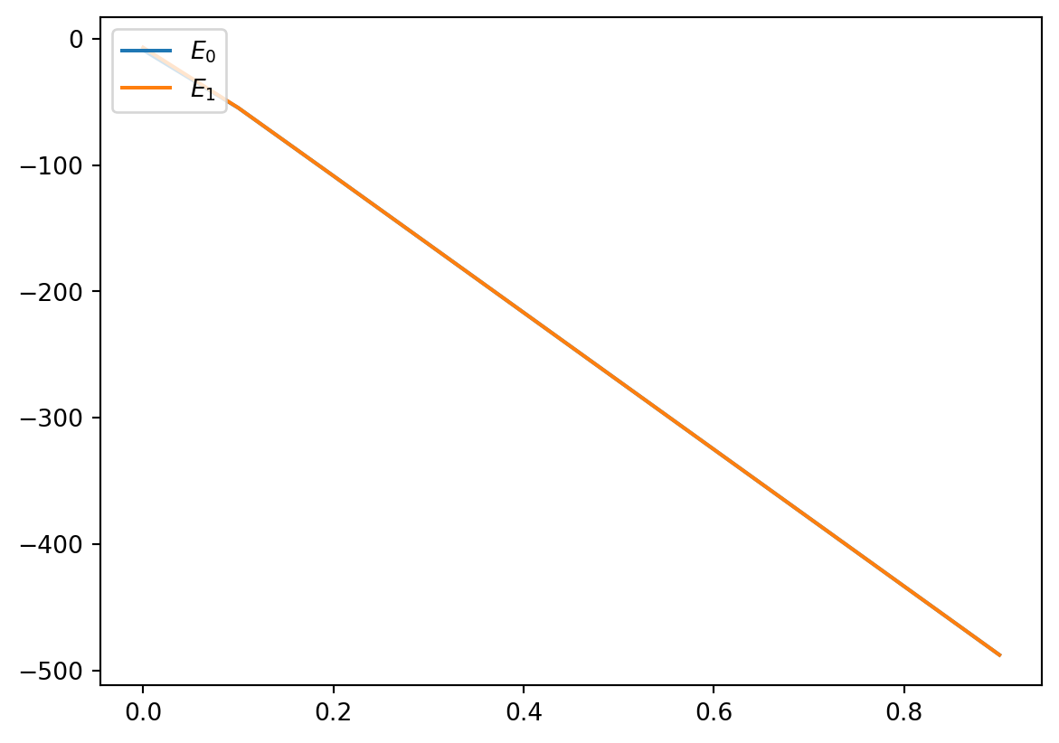
We it sounds that we are working with a really small gap in this setup, not a good option if we would like use adiabatic computing as we saw before. We could of course, once there is a quantum mechanical procedure, implement it using a digitized approach.
from qiskit import QuantumCircuit

initial_state = QuantumCircuit(size)

# Hadamard gate
for qb_i in initial_state.qubits:
    initial_state.h(qb_i)
initial_state.draw('mpl')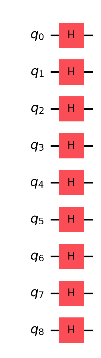
from qiskit.circuit import Parameter

# Create a parameter to instantiate
beta = Parameter("$\\beta$")

mixer = QuantumCircuit(size,size)
for i in range(size):
    mixer.rx(2*beta*(-1), i)

mixer.draw('mpl')
from qiskit.circuit import Parameter

# Create a parameter to instantiate
gamma = Parameter("$\\gamma$")

problem = QuantumCircuit(size,size)

for node, h_val in enumerate(hp):
    problem.rz(2*gamma*h_val, node)

for key in jp:
    problem.rzz(2*gamma*jp[key], key[0], key[1])

problem.draw('mpl', fold=-1)
With these three blocks we just need to define how we are going to digitize the evolution towards the solution to our problem.
tsp_circ = QuantumCircuit(size,size)
tsp_circ.compose(initial_state, inplace=True)

# Length of the equidistant steps
dt = 0.1

for lt in np.arange(0.1, 1.1, dt):
    tsp_circ.compose(problem.assign_parameters({gamma: lt}), inplace=True)
    tsp_circ.compose(mixer.assign_parameters({beta: (1-lt)}), inplace=True)
tsp_circ.measure(range(size), range(size))

tsp_circ.draw('mpl', fold=500)
Get’s harder to see. We can check for that evolution the final response but also some interesting features like circuit depth or number of operations, which will become relevant when trying to quantify the accuracy of our simulation associated with a given device noise/error.
tsp_circ.depth()118tsp_circ.num_nonlocal_gates()360Let’s simulate the distribution…
from qiskit_aer import AerSimulator
from qiskit.visualization import plot_histogram

# execute the quantum circuit
backend = AerSimulator()

# execute the quantum circuit
result = backend.run(tsp_circ, shots=10_000).result()
counts  = result.get_counts(tsp_circ)

plot_histogram(counts)
And its energy profile…
energy = []
success_probability = []

for bit_string in counts:
    solution = [int(char) for char in bit_string]
    solution_dict = {}
    for i, v in enumerate(indexes):
        solution_dict[v] = solution[i]
    energy.append(bqm.energy(solution_dict))
    success_probability.append(counts[bit_string]/10_000)

plt.bar(energy, height=success_probability, label="Digitized AQC")
plt.show()
We can definitely improve this towards a left-skewed version but we would need to find the right scheduling for it.