Appendix D — Interesting characteristics

D.1 Expressivity

One simple approach is to compare the distribution of fidelities obtainer from sampling \(n\) number of times with randomly selected parameters given a target PQC to be evaluated in comparison with the uniform distribution of fidelities for the same domain, like the ensemble of Haar random states.

Thus, \[ \text{Expr} = D_{KL}\left( \hat{P}_{PQC}(F; \theta) \| P_{Haar}(F)\right) = \sum_{j} \hat{P}_{PQC}(F_j; \theta)\log\left(\frac{\hat{P}_{PQC}(F_j; \theta)}{P_{\text{Haar}(F_j)}}\right) \]

where \(\hat{P}_{PQC}(F; \theta)\) is the estimated probability distribution of fidelities resulting while sampling states from a PQC with parameters \(\theta\). \(F_j\) represents the fidelity at \(j\)th bin.

Thus, we need to generate a histogram of the elements of \(F\). The output of this histogram is a set of bins \(B = \{(l_1, u_1), (l_2, u_2), \cdots \}\) where \(l_{j}\) (\(u_j\)) denotes the lower (upper) limit of bin \(j\). It also produces an empirical probability distribution function \(\mathrm{P}_{\text{PQC}}(j)\), which is simply the probability that a given value of \(F\) falls in a bin \(j\).

Let’s take the ansatz defined by an idle circuit as an example.

from qiskit import QuantumCircuit

qc = QuantumCircuit(1, 1)

qc.draw('mpl')

from qiskit.quantum_info import Statevector
from qiskit.visualization import plot_bloch_multivector

psi  = Statevector.from_instruction(qc)
plot_bloch_multivector(psi)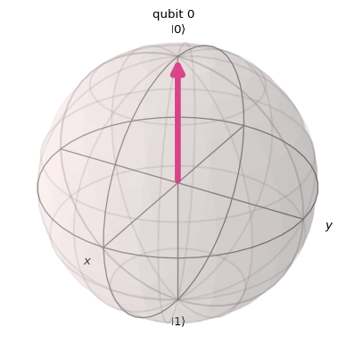

No matter what we do, the ansatz won’t change, therefore its expressivity should be equal to none.

import numpy as np
import matplotlib.pyplot as plt
from qiskit_aer import AerSimulator

# Size of our histogram
dims = 100
num_qubits = 1

# Possible Bin
bins_list = []
for i in range(dims):
    bins_list.append((i) / (dims - 1))

# Harr histogram
p_haar_hist = []
for i in range(dims - 1):
    p_haar_hist.append(
        (1 - bins_list[i]) ** (2**num_qubits - 1) - (1 - bins_list[i + 1]) ** (2**num_qubits - 1)
    )

# Select the AerSimulator from the Aer provider
simulator = AerSimulator(method='matrix_product_state')

# Sample from circuit
nshot=1_024
nsamples=1_000
fidelities=[]    
for _ in range(nsamples):
    qc = QuantumCircuit(1, 1)
    qc.measure(0,0)

    job = simulator.run([qc], shots = nshot)
    result = job.result()
    count = result.get_counts()

    # Fidelity
    if '0' in count:
        ratio=count['0']/nshot
    else:
        ratio=0
    fidelities.append(ratio)

weights = np.ones_like(fidelities) / float(len(fidelities))

# Plot
bins_x = []
for i in range(dims - 1):
    bins_x.append(bins_list[1] + bins_list[i])

plt.hist(
    fidelities,
    bins=bins_list,
    weights=weights,
    label="Circuit",
    range=[0, 1],
)
plt.plot(bins_x, p_haar_hist, label="Haar")
plt.legend(loc="upper right")
plt.show()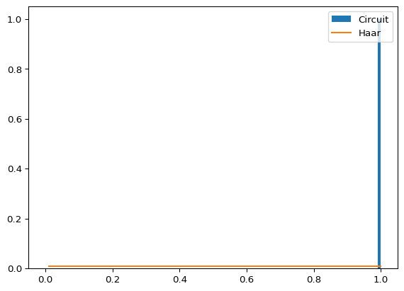

Zero means maximal expressivity

We can see how all fidelities are probability of zero except for fidelity 1, which means there is only one state we can render with this circuit. The expressivity works backwards, meaning a distance of zero represents the fidelity probability landscape equal to the uniform distribution. Therefore, all states (pure) in the Hilbert space can be produced with the right set of parameters (\(\theta\)). Thus the expressivity will take the maximum value as the \(log(N)\) where \(N\) is the number of bins selected for the histogram.

from scipy.special import rel_entr # For entropy calculation

pi_hist = np.histogram(fidelities, bins=bins_list, weights=weights, range=[0, 1])[0]
print("Expr = ", sum(rel_entr(pi_hist, p_haar_hist)))

Expr =  4.595119850134598

This will numerically approximate the value of

np.log(dims)

np.float64(4.605170185988092)

hence, 0 is the maximum expressivity we can get.

We can see what would be the effect if we introduce a parameterized gate instead, something more complex with a free parameter such as:

from qiskit import QuantumCircuit
from qiskit.circuit import Parameter

a = Parameter('a')

qc = QuantumCircuit(1, 1)
qc.h(0)
qc.rz(a, 0)

qc.draw('mpl')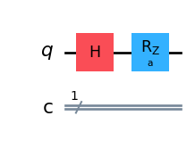

from random import random

# Possible Bin
bins_list = []
for i in range(dims):
    bins_list.append((i) / (dims - 1))

# Haar histogram
p_haar_hist = []
for i in range(dims - 1):
    p_haar_hist.append(
        (1 - bins_list[i]) ** (2**num_qubits - 1) - (1 - bins_list[i + 1]) ** (2**num_qubits - 1)
    )

# Select the AerSimulator from the Aer provider
simulator = AerSimulator(method='matrix_product_state')

# Sample from circuit
fidelities=[]    
for _ in range(nsamples):
    qc = QuantumCircuit(1, 1)
    qc.h(0)
    qc.rz(2 * np.pi * random(), 0)
    # Inverse of the circuit
    qc.rz(2 * np.pi * random(), 0)
    qc.h(0)
    qc.measure(0,0)

    job = simulator.run([qc], shots = nshot)
    result = job.result()
    count = result.get_counts()

    # Fidelity
    if '0' in count:
        ratio=count['0']/nshot
    else:
        ratio=0
    fidelities.append(ratio)

weights = np.ones_like(fidelities) / float(len(fidelities))

# Plot
bins_x = []
for i in range(dims - 1):
    bins_x.append(bins_list[1] + bins_list[i])

plt.hist(
    fidelities,
    bins=bins_list,
    weights=weights,
    label="Circuit",
    range=[0, 1],
)
plt.plot(bins_x, p_haar_hist, label="Haar")
plt.legend(loc="upper right")
plt.show()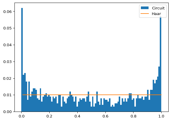

pi_hist = np.histogram(fidelities, bins=bins_list, weights=weights, range=[0, 1])[0]
print("Expr = ", sum(rel_entr(pi_hist, p_haar_hist)))

Expr =  0.21766234960533026

We can extend this acting on more than one axis, which should end up with the maximum coverage over the bloch sphere for this one single qubit case.

from qiskit import QuantumCircuit
from qiskit.circuit import Parameter

a = Parameter('a')
b = Parameter('b')

qc = QuantumCircuit(1, 1)
qc.h(0)
qc.rz(a, 0)
qc.rx(b, 0)

qc.draw('mpl')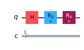

# Possible Bin
bins_list = []
for i in range(dims):
    bins_list.append((i) / (dims - 1))

# Haar histogram
p_haar_hist = []
for i in range(dims - 1):
    p_haar_hist.append(
        (1 - bins_list[i]) ** (2**num_qubits - 1) - (1 - bins_list[i + 1]) ** (2**num_qubits - 1)
    )

# Select the AerSimulator from the Aer provider
simulator = AerSimulator(method='matrix_product_state')

# Sample from circuit
fidelities=[]    
for _ in range(nsamples):
    qc = QuantumCircuit(1, 1)
    qc.h(0)
    qc.rz(2 * np.pi * random(), 0)
    qc.rx(2 * np.pi * random(), 0)
    # Inverse of the circuit
    qc.rx(2 * np.pi * random(), 0)
    qc.rz(2 * np.pi * random(), 0)
    qc.h(0)
    qc.measure(0,0)

    job = simulator.run([qc], shots = nshot)
    result = job.result()
    count = result.get_counts()

    # Fidelity
    if '0' in count:
        ratio=count['0']/nshot
    else:
        ratio=0
    fidelities.append(ratio)

weights = np.ones_like(fidelities) / float(len(fidelities))

# Plot
bins_x = []
for i in range(dims - 1):
    bins_x.append(bins_list[1] + bins_list[i])

plt.hist(
    fidelities,
    bins=bins_list,
    weights=weights,
    label="Circuit",
    range=[0, 1],
)
plt.plot(bins_x, p_haar_hist, label="Haar")
plt.legend(loc="upper right")
plt.show()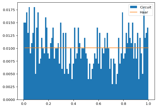

pi_hist = np.histogram(fidelities, bins=bins_list, weights=weights, range=[0, 1])[0]
print("Expr = ", sum(rel_entr(pi_hist, p_haar_hist)))

Expr =  0.06728209189372705

These plots should resemble those at the original work (Sim, Johnson, and Aspuru-Guzik 2019).

Sim, Sukin, Peter D Johnson, and Alán Aspuru-Guzik. 2019. “Expressibility and Entangling Capability of Parameterized Quantum Circuits for Hybrid Quantum-Classical Algorithms.” Advanced Quantum Technologies 2 (12): 1900070.