AQC in practice

We will make a simple example so that the formalism of this algorithm is clear to everyone. We will need for this exercise:

• A initial Hamiltonian and its ground state
• A final Hamiltonian
• A Scheduling function that governs the evolution and mixture between the two

So let’s start by selecting our initial Hamiltonian:

\[ H_{init} = - \sum_i^N \sigma_i^x \]

N = 3 # 4 qubit system

import numpy as np

sigma_x = np.matrix([[0, 1],
                     [1, 0]])

H_init = 0
for j in range(N):
    H_init += -1.0 * np.kron( np.kron(np.identity(2**j), sigma_x), np.identity(2**(N-j-1)) )

H_init

matrix([[ 0., -1., -1.,  0., -1.,  0.,  0.,  0.],
        [-1.,  0.,  0., -1.,  0., -1.,  0.,  0.],
        [-1.,  0.,  0., -1.,  0.,  0., -1.,  0.],
        [ 0., -1., -1.,  0.,  0.,  0.,  0., -1.],
        [-1.,  0.,  0.,  0.,  0., -1., -1.,  0.],
        [ 0., -1.,  0.,  0., -1.,  0.,  0., -1.],
        [ 0.,  0., -1.,  0., -1.,  0.,  0., -1.],
        [ 0.,  0.,  0., -1.,  0., -1., -1.,  0.]])

Now we will use a couple of functions to compute the Eigenspectra (set of eigenvalues for a given Hamiltonian) and the ground-state (minimum energy state).

from math import sqrt
from numpy.linalg import eig

def get_eigenspectra(h_mat):
    """
    Computes the eigenspectra
    """
    evals, evecs = eig(h_mat)
    sort_index = np.argsort(evals)

    return evals [sort_index], evecs[:, sort_index]

def get_gs(h_mat):
    """ Computes the ground state """
    evals, evecs = eig(h_mat)
    sort_index = np.argsort(evals)

    stat_gs = evecs[:, sort_index[0]]
    gs_val = evals[sort_index[0]]
    
    num = 1
    for idx in sort_index[1:]:
        if evals[idx] == gs_val:
            stat_gs += evecs[:, idx]
            num += 1
        else:
            break

    return np.dot((1/sqrt(num)), stat_gs)

So, by computing the ground state of our initial Hamiltonian we can check that it is the superposition of all possible states with equal probability.

get_gs(H_init)

matrix([[-0.35355339],
        [-0.35355339],
        [-0.35355339],
        [-0.35355339],
        [-0.35355339],
        [-0.35355339],
        [-0.35355339],
        [-0.35355339]])

Now for our target Hamiltonian we will select a random instance of the Ising model that looks like:

\[ H_{problem} = \sum_j^N J_{j,j+1}\sigma_j^z\sigma_{j+1}^z \]

J = -1

sigma_z = np.matrix([[1, 0],
                     [0, -1]])

H_problem = 0
for i in range(N-1):
    H_problem = J* np.kron( np.kron(np.identity(2**i), sigma_z), np.identity(2**(N-i-1)) ) * np.kron( np.kron(np.identity(2**(i+1)), sigma_z), np.identity(2**(N-(i+1)-1)) )

H_problem

matrix([[-1.,  0.,  0.,  0.,  0.,  0.,  0.,  0.],
        [ 0.,  1.,  0.,  0.,  0.,  0.,  0.,  0.],
        [ 0.,  0.,  1.,  0.,  0.,  0.,  0.,  0.],
        [ 0.,  0.,  0., -1.,  0.,  0.,  0.,  0.],
        [ 0.,  0.,  0.,  0., -1.,  0.,  0.,  0.],
        [ 0.,  0.,  0.,  0.,  0.,  1.,  0.,  0.],
        [ 0.,  0.,  0.,  0.,  0.,  0.,  1.,  0.],
        [ 0.,  0.,  0.,  0.,  0.,  0.,  0., -1.]])

get_gs(H_problem)

matrix([[0.5],
        [0. ],
        [0. ],
        [0.5],
        [0.5],
        [0. ],
        [0. ],
        [0.5]])

We can see our Ising model has a ground state looking like

\[ |\psi\rangle = \frac{1}{2}|000\rangle + \frac{1}{2}|011\rangle + \frac{1}{2}|100\rangle + \frac{1}{2}|111\rangle. \]

Now we would only need to define a scheduling function to mix both Hamiltonians. Just for simplicity we will use a single scheduling function \(\lambda(t)\) and use its complementary for the decaying of the initial Hamiltonian.

\[ H(t) = (1-\lambda(t))H_{init} + \lambda(t)H_{problem} \]

e0 = []
e1 = []
time_range = np.arange(0.0, 1.0, 0.1)

for lambda_t in time_range:

    H = (1-lambda_t)*H_init + lambda_t*H_problem

    vals, stats = get_eigenspectra(H)
    e0.append(vals[0])
    e1.append(vals[1])

import matplotlib.pyplot as plt

plt.plot(time_range, e0, time_range, e1)
plt.show()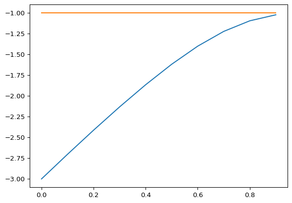

plt.plot(np.subtract(e1,e0))
plt.show()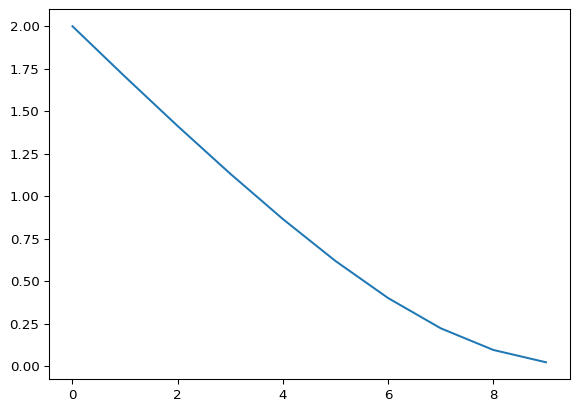

stats[:, 0]

matrix([[0.49701447],
        [0.05455839],
        [0.05455839],
        [0.49701447],
        [0.49701447],
        [0.05455839],
        [0.05455839],
        [0.49701447]])

There you go, the obtained state corresponds with the desired

\[ |\psi\rangle = \frac{1}{2}|000\rangle + \frac{1}{2}|011\rangle + \frac{1}{2}|100\rangle + \frac{1}{2}|111\rangle. \]

up to a precision.