from qiskit import QuantumCircuit

qc = QuantumCircuit(2, 2)
qc.h(0)
qc.h(1)

qc.draw('mpl')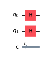
You may wonder, do we use the complex part at all? So far, I haven’t seen any usage of it. Well, we do. In fact it is key to many of the algorithms we unlock with quantum computing. Moving around the X-axis of the bloch sphere and acting upon it.
Let’s take an example on a superposed state.
from qiskit import QuantumCircuit
qc = QuantumCircuit(2, 2)
qc.h(0)
qc.h(1)
qc.draw('mpl')
from qiskit.quantum_info import Statevector
from qiskit.visualization import plot_bloch_multivector

psi  = Statevector.from_instruction(qc)
plot_bloch_multivector(psi)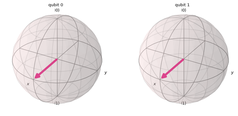
What is that state, we can check its mathematical formulation which end up being
\[ |\psi\rangle = \frac{1}{2}\left(|00\rangle + |01\rangle + |10\rangle +|11\rangle\right) \]
from qiskit.visualization import array_to_latex

array_to_latex(array=psi, prefix='|\\psi\\rangle = ', max_size=(10,10))
\[ |\psi\rangle = \begin{bmatrix} \frac{1}{2} & \frac{1}{2} & \frac{1}{2} & \frac{1}{2} \\ \end{bmatrix} \]
Go and extend the circuit… and check what happens.
import numpy as np

qc.ry(np.pi/2, 1)

qc.draw('mpl')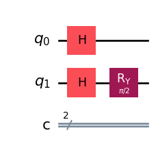
psi  = Statevector.from_instruction(qc)
plot_bloch_multivector(psi)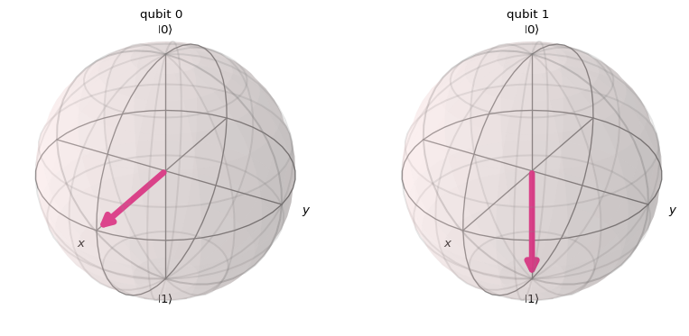
from qiskit.visualization import array_to_latex

array_to_latex(array=psi, prefix='|\\psi\\rangle = ', max_size=(10,10))
\[ |\psi\rangle = \begin{bmatrix} 0 & 0 & \frac{\sqrt{2}}{2} & \frac{\sqrt{2}}{2} \\ \end{bmatrix} \]
Ok, so now we have the following shape \[ |\psi\rangle = |1\rangle \otimes \frac{\sqrt{2}}{2}\left(|0\rangle + |1\rangle\right) = |1+\rangle \]
which shows a state where one qubit is in the 1 state (all odds into reading the 1 value int he computational basis), while the other qubit looks still in a superposition (50-50 chances of getting 0 or 1 in the computational basis). As we mentioned before, this is not an entangled state as it is separable. Hence, the tensor product symbol.
You found weird the state was \(|1+\rangle\) instead of \(|+1\rangle\) ? You are not alone, check this entry by Lukasz Palt for further clarification.
Now, look what happens when we act on the second qubit controlled by the first one.
import numpy as np

qc.crz(np.pi, 0, 1)

qc.draw('mpl')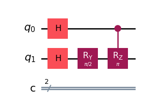
psi  = Statevector.from_instruction(qc)
plot_bloch_multivector(psi)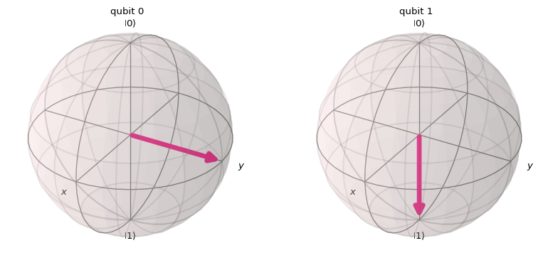
The Z-rotation on the target qubit had almost no effect, but what happened to the control one? It moved?
from qiskit.visualization import array_to_latex

array_to_latex(array=psi, prefix='|\\psi\\rangle = ', max_size=(10,10))
\[ |\psi\rangle = \begin{bmatrix} 0 & 0 & \frac{\sqrt{2}}{2} & \frac{\sqrt{2} i}{2} \\ \end{bmatrix} \]
Wait, there is a \(i\) in there? Yeap. We changed the phase of one of the elements in the control qubit. It is not only in between 0 and 1 poles, but also we added a phase to it that is represented by the sign direction in the complex axis.
\[ |\psi\rangle = |1\rangle \otimes \frac{\sqrt{2}}{2}\left(|0\rangle + e^{i\pi/2}|1\rangle\right) = |1+\rangle \]
np.round(psi.data,2)array([0. +0.j , 0. -0.j , 0.71+0.j , 0. +0.71j])That is the effect when the phase \(e^{i\pi/2}\) gets applied then.
np.round(np.exp(1j*np.pi/2)/np.sqrt(2), 2)np.complex128(0.71j)Really interesting. In fact, this is the effect behind many of the theoretical works related to the speedup of solving systems of linear equations, for example (Harrow et al. 2009).
This is a great resource going deep in some of the algorithms that use this effect
And for those that prefer Pennylane or reading about it, this is a great tutorial on the basics on how phase allows as to identify specific states in our search sapce.