import networkx as nx

# Create empty graph
G = nx.Graph()

# Add edges to the graph (also adds nodes)
G.add_edges_from([(1,2),(1,3),(2,4),(3,4),(3,5),(4,5)])

nx.draw(G)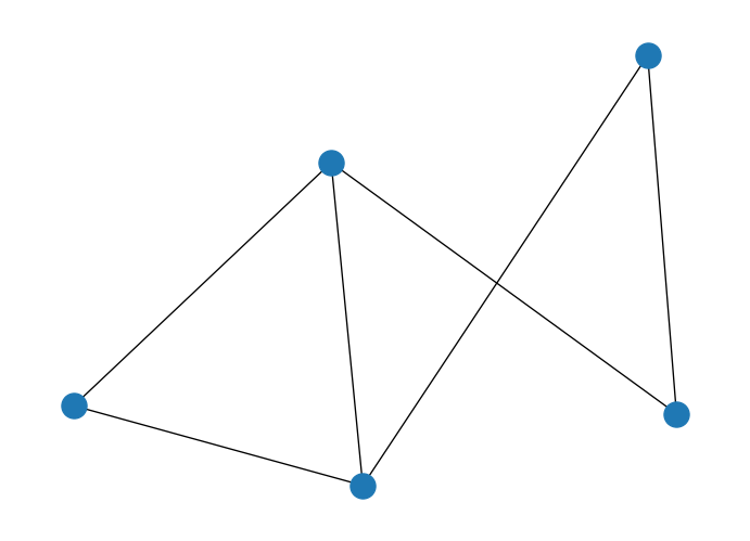
We will use our previous example on MaxCut just to take it simple.
import networkx as nx
# Create empty graph
G = nx.Graph()
# Add edges to the graph (also adds nodes)
G.add_edges_from([(1,2),(1,3),(2,4),(3,4),(3,5),(4,5)])
nx.draw(G)
from collections import defaultdict

# Initialize our Q matrix
Q = defaultdict(int)

# Update Q matrix for every edge in the graph
for i, j in G.edges:
    Q[(i,i)]+= -1
    Q[(j,j)]+= -1
    Q[(i,j)]+= 2
from dimod import ExactSolver
# Set up QPU parameters
chainstrength = 8
numruns = 10
# Run the QUBO on the solver from your config file
sampler = ExactSolver()
response = sampler.sample_qubo(Q)print('-' * 60)
print('{:>15s}{:>15s}{:^15s}{:^15s}'.format('Set 0','Set 1','Energy','Cut Size'))
print('-' * 60)
for sample, E in response.data(fields=['sample','energy']):
S0 = [k for k,v in sample.items() if v == 0]
S1 = [k for k,v in sample.items() if v == 1]
print('{:>15s}{:>15s}{:^15s}{:^15s}'.format(str(S0),str(S1),str(E),str(int(-1*E))))------------------------------------------------------------
Set 0 Set 1 Energy Cut Size
------------------------------------------------------------
[1, 4, 5] [2, 3] -5.0 5
[2, 3, 5] [1, 4] -5.0 5
[1, 4] [2, 3, 5] -5.0 5
[2, 3] [1, 4, 5] -5.0 5
[2, 5] [1, 3, 4] -4.0 4
[2, 3, 4] [1, 5] -4.0 4
[1, 2, 5] [3, 4] -4.0 4
[1, 5] [2, 3, 4] -4.0 4
[3, 4] [1, 2, 5] -4.0 4
[1, 3, 4] [2, 5] -4.0 4
[1, 2, 3, 5] [4] -3.0 3
[1, 3, 5] [2, 4] -3.0 3
[3, 5] [1, 2, 4] -3.0 3
[1, 2, 4, 5] [3] -3.0 3
[4, 5] [1, 2, 3] -3.0 3
[2, 4, 5] [1, 3] -3.0 3
[4] [1, 2, 3, 5] -3.0 3
[2, 4] [1, 3, 5] -3.0 3
[1, 2, 4] [3, 5] -3.0 3
[1, 3] [2, 4, 5] -3.0 3
[3] [1, 2, 4, 5] -3.0 3
[1, 2, 3] [4, 5] -3.0 3
[3, 4, 5] [1, 2] -2.0 2
[1, 3, 4, 5] [2] -2.0 2
[2] [1, 3, 4, 5] -2.0 2
[5] [1, 2, 3, 4] -2.0 2
[2, 3, 4, 5] [1] -2.0 2
[1] [2, 3, 4, 5] -2.0 2
[1, 2, 3, 4] [5] -2.0 2
[1, 2] [3, 4, 5] -2.0 2
[1, 2, 3, 4, 5] [] 0.0 0
[][1, 2, 3, 4, 5] 0.0 0 from qiskit.visualization import plot_histogram
solution = {
'01101': 0.25,
'10010': 0.25,
'10011': 0.25,
'01100': 0.25,
}
plot_histogram(solution)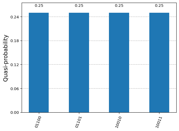
Ok, we don’t always know the solution in advance but it is important for educational purposes. Let’s take the three pieces from our digitized AQC and built block by block, starting by the quantum state that is the ground state of our \(H_{init}=-\sum_n \sigma_i^n\)
from qiskit import QuantumCircuit

size = G.number_of_nodes()

initial_state = QuantumCircuit(size)

# Hadamard gate
for qb_i in initial_state.qubits:
    initial_state.h(qb_i)
initial_state.draw('mpl')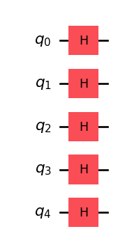
This is simple and we can check the output of that actual circuit. Check out how the distribution resolution changes depending on the shots parameters.
from qiskit_aer import AerSimulator

qc = QuantumCircuit(size, size)
qc = qc.compose(initial_state)

# Measures added
qc.measure(range(size), range(size))

# execute the quantum circuit
backend = AerSimulator()
result = backend.run(qc, shots=10000).result()
counts  = result.get_counts(qc)

plot_histogram(counts)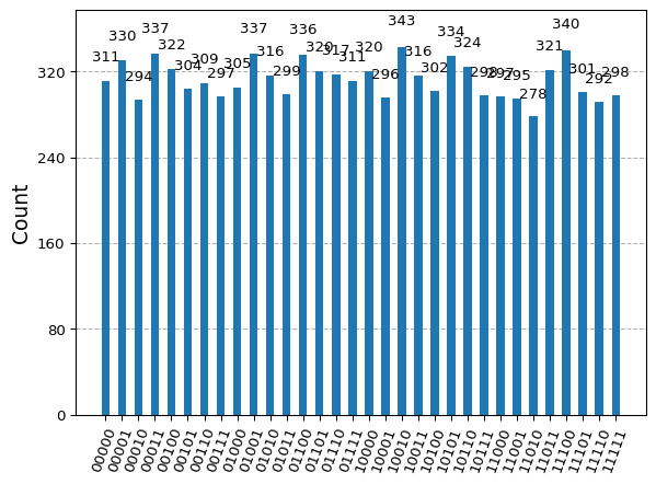
import qiskit.quantum_info as qi

psi = qi.Statevector.from_instruction(initial_state)
psi.draw('latex', prefix='|\\psi\\rangle = ')
\[|\psi\rangle = 0.1767766953 |00000\rangle+0.1767766953 |00001\rangle+0.1767766953 |00010\rangle+0.1767766953 |00011\rangle+0.1767766953 |00100\rangle+0.1767766953 |00101\rangle + \ldots +0.1767766953 |11011\rangle+0.1767766953 |11100\rangle+0.1767766953 |11101\rangle+0.1767766953 |11110\rangle+0.1767766953 |11111\rangle\]
from qiskit.visualization import plot_bloch_multivector

plot_bloch_multivector(psi)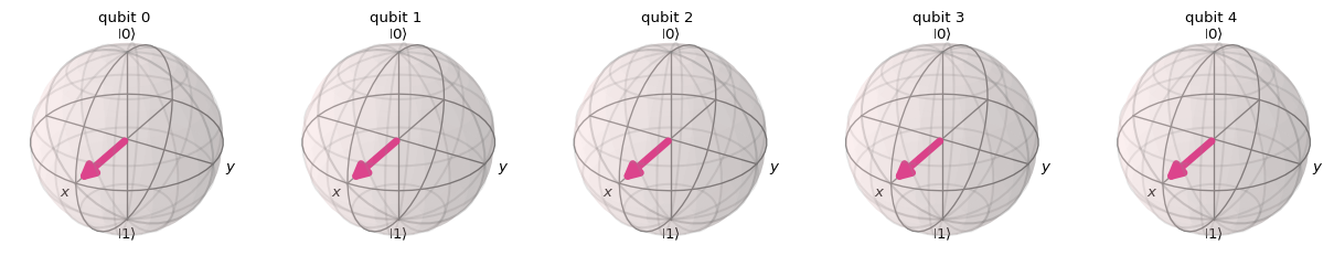
Ok so the starting point is just simply all potential solutions: \(|+\rangle^{\otimes n}\)
Now we can add the blocks for \(H_{init}\) and \(H_{problem}\).
from qiskit.circuit import Parameter

# Create a parameter to instantiate
beta = Parameter("$\\beta$")

mixer = QuantumCircuit(size,size)
for i in range(size):
    mixer.rx(2*beta*(-1), i)

mixer.draw('mpl')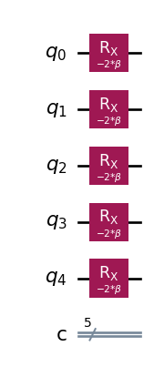
This following code is a particular version of the MaxCut instance as in a fully informed Ising model we would need to add \(Z\) rotations depending on the weight of the node and \(ZZ\) rotations accoding to coupling strengh of each edge. But given that we have a sparse matrix, we can take advantage of that.
import numpy as np

H_problem = np.zeros((size, size))

for k, v in Q.items():
    if not isinstance(k, int):
        H_problem[k[0]-1][k[1]-1] = v

H_problem
array([[-2., 2., 2., 0., 0.],
[ 0., -2., 0., 2., 0.],
[ 0., 0., -3., 2., 2.],
[ 0., 0., 0., -3., 2.],
[ 0., 0., 0., 0., -2.]])from qiskit.circuit import Parameter
# Create a parameter to instantiate
gamma = Parameter("$\\gamma$")
problem = QuantumCircuit(size,size)
for node in range(size):
problem.rz(2*gamma*H_problem[node][node], node)
for node_i in range(size):
for node_j in range(node_i + 1, size):
if H_problem[node_i][node_j] > 0:
problem.rzz(2*gamma*H_problem[node_i][node_j], node_i, node_j)
problem.draw('mpl')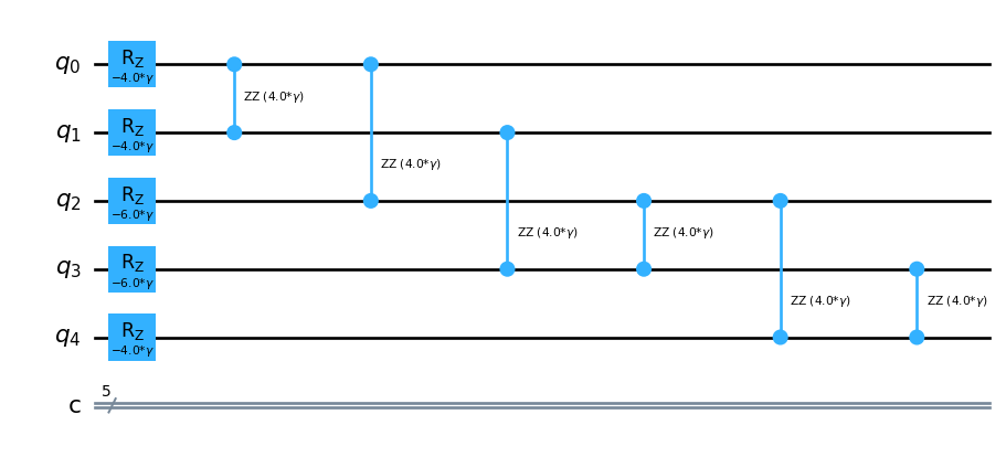
We have the three main blocks for setting our digitized version of the problem. Now we need to define a composition for those blocks where:
Wbeing \(n\) the number of trotter steps. We can do a first approach with a simple stepwise linear approach.
maxcut = QuantumCircuit(size,size)
maxcut.compose(initial_state, inplace=True)

dt = 0.1

for lt in np.arange(0.1, 1.1, dt):
    maxcut.compose(problem.assign_parameters({gamma: lt}), inplace=True)
    maxcut.compose(mixer.assign_parameters({beta: (1-lt)}), inplace=True)
maxcut.measure(range(size), range(size))
maxcut.draw('mpl', fold=500)
# execute the quantum circuit
result = backend.run(maxcut, shots=10000).result()
counts  = result.get_counts(maxcut)

plot_histogram(counts)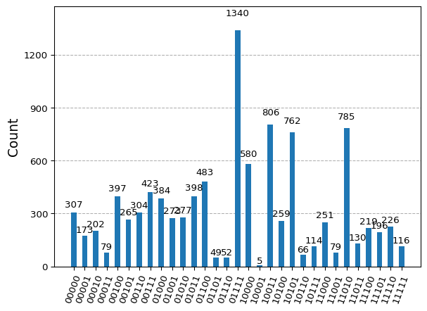
import matplotlib.pyplot as plt

energy = []
success_probability = []

for bit_string in counts:
    solution = [int(char) for char in bit_string]
    energy.append(np.dot(np.transpose(solution), np.dot(H_problem, solution)))
    success_probability.append(counts[bit_string]/10000)

plt.bar(energy, height=success_probability, label="Digitized AQC")
plt.show()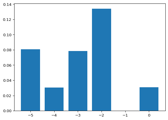
Let’s increase the schedule so that slower evolution is considered.
maxcut = QuantumCircuit(size,size)
maxcut.compose(initial_state, inplace=True)

dt = 0.01

for lt in np.arange(0.1, 1.1, dt):
    maxcut.compose(problem.assign_parameters({gamma: lt}), inplace=True)
    maxcut.compose(mixer.assign_parameters({beta: (1-lt)}), inplace=True)
maxcut.measure(range(size), range(size))
maxcut.draw('mpl', fold=500)
result = backend.run(maxcut, shots=10000).result()
counts  = result.get_counts(maxcut)

plot_histogram(counts)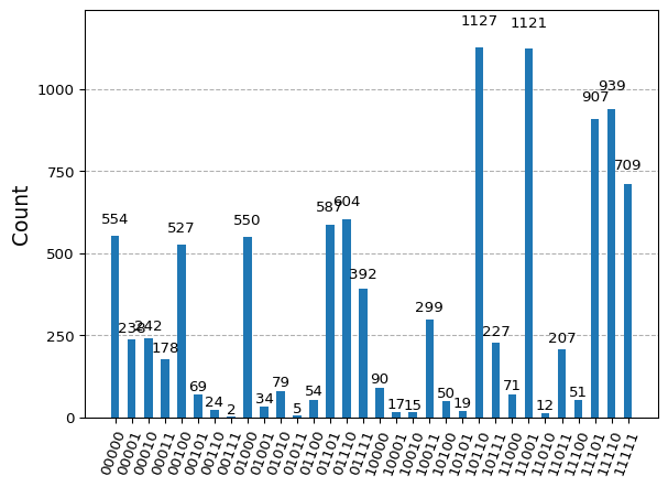
energy = []
success_probability = []

for bit_string in counts:
    solution = [int(char) for char in bit_string]
    energy.append(np.dot(np.transpose(solution), np.dot(H_problem, solution)))
    success_probability.append(counts[bit_string]/10000)

plt.bar(energy, height=success_probability, label="Digitized AQC")
plt.show()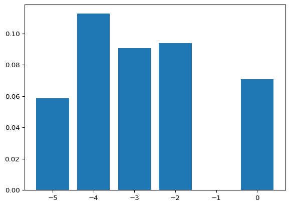
We could select a much more efficient scheduling function, but we should look into the energy evolution, the gap… let’s take a wild guess.
def scheduling_function(t, T):

    return np.sin((np.pi/2)*np.sin((np.pi * t)/(2*T))**2)**2
T = 1.0
dt = 0.1
timeline = np.arange(0.1, T, dt)
val = [scheduling_function(t, T) for t in timeline]plt.plot(timeline, val, label="Schedule")
plt.show()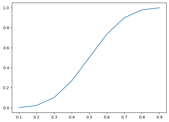
maxcut = QuantumCircuit(size,size)
maxcut.compose(initial_state, inplace=True)

T = 1.0
dt = 0.1

timeline = np.arange(0.1, T, dt)

for t in np.arange(0.1, T, dt):
    lambda_t = scheduling_function(t, T)
    maxcut.compose(problem.assign_parameters({gamma: dt*lambda_t}), inplace=True)
    maxcut.compose(mixer.assign_parameters({beta: dt*(1-lambda_t)}), inplace=True)
maxcut.measure(range(size), range(size))
maxcut.draw('mpl', fold=500)
result = backend.run(maxcut, shots=10000).result()
counts  = result.get_counts(maxcut)

plot_histogram(counts)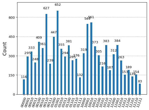
energy = []
success_probability = []

for bit_string in counts:
    solution = [int(char) for char in bit_string]
    energy.append(np.dot(np.transpose(solution), np.dot(H_problem, solution)))
    success_probability.append(counts[bit_string]/10000)

plt.bar(energy, height=success_probability, label="Digitized AQC")
plt.show()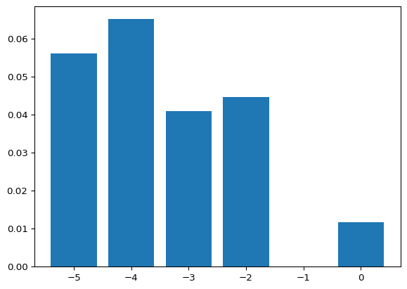
Getting close…
maxcut = QuantumCircuit(size,size)
maxcut.compose(initial_state, inplace=True)

T = 5.0
dt = 0.05

timeline = np.arange(0.1, T, dt)

for t in np.arange(0.1, T, dt):
    lambda_t = scheduling_function(t, T)
    maxcut.compose(problem.assign_parameters({gamma: dt*lambda_t}), inplace=True)
    maxcut.compose(mixer.assign_parameters({beta: dt*(1-lambda_t)}), inplace=True)
maxcut.measure(range(size), range(size))
maxcut.draw('mpl', fold=500)
result = backend.run(maxcut, shots=10000).result()
counts  = result.get_counts(maxcut)

plot_histogram(counts)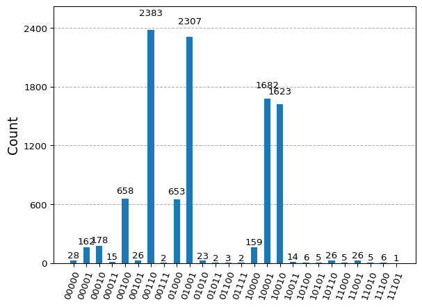
energy = []
success_probability = []

for bit_string in counts:
    solution = [int(char) for char in bit_string]
    energy.append(np.dot(np.transpose(solution), np.dot(H_problem, solution)))
    success_probability.append(counts[bit_string]/10000)

plt.bar(energy, height=success_probability, label="Digitized AQC")

plt.show()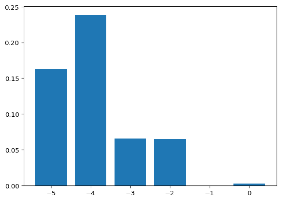
Let’s play around a bit with the time parameters and see if we get a good concentration of -5 energy states. Ideally our sampling from the ground state should be below \(2^5 = 32\) samples, otherwise, brute forcing would be more efficient in this cases. But in absence of knowledge we should guess for a while.
We could rely on techniques known to be used to find parameters in a model. Yeah, machine learning techniques.