Feature maps

Feature maps are the way in which classical data gets transformed into quantum states. A good point to start is to use existing templates from libraries like Pennylane.

Basis encoding

Basis encoding might be one of the most simplistic ways to map classical data in quantum states. It requires our data to be composed by integers and maps its binary representation to the basis state that maps the same binary string: \(n = 4, \quad b_n = 1001, \quad |b_n\rangle = |1001\rangle\).

\[ |X\rangle = \frac{1}{\sqrt{M}}\sum_{m=1}^M |x^m \rangle \]

It is not often used as it limits the data that can be embedded and requires quite some resources from the quantum side which are not fully utilized.

import pennylane as qml
from qiskit.visualization import array_to_latex

dev = qml.device('default.qubit', wires=3)

@qml.qnode(dev)
def feature_map(feature_vector):
    qml.BasisEmbedding(features=feature_vector, wires=range(3))
    return qml.state()

X = [1,1,1]

array_to_latex(array=feature_map(X).T, prefix='| \\psi \\rangle = ', max_size=(10,10))

\[ | \psi \rangle = \begin{bmatrix} 0 & 0 & 0 & 0 & 0 & 0 & 0 & 1 \\ \end{bmatrix} \]

Angle encoding

Angle encoding takes benefit from the ability to embed rotation angles into our gates so that we can introduce our numeric data as the rotation angle of a given qubit. Example, \(x = [x_1, x_2,...,x_n]\) would be mapped to

\[ (R_x(x_1) \otimes R_x(x_2) \otimes \dots \otimes R_x(x_n))|0\rangle^{\otimes n} \]

data must be in the regime where those rotations take effect (\([0, 2\pi]\)) and may be more suitable if a cyclic nature is already present. Normalization of data may be relevant preprocessing step in this case.

import pennylane as qml
import pennylane.numpy as np

dev = qml.device('default.qubit', wires=3)

@qml.qnode(dev)
def feature_map(feature_vector):
    qml.AngleEmbedding(features=feature_vector, wires=range(3), rotation='Z')
    return qml.state()

X = [2*np.pi,0,np.pi]

print(qml.draw(feature_map, level="device")(X))

0: ──RZ(6.28)─┤ ╭State
1: ──RZ(0.00)─┤ ├State
2: ──RZ(3.14)─┤ ╰State

Amplitude encoding

Amplitude encoding takes the probability amplitude of elements on an array and matches those to the position the where placed at. Assuming our data is composed by \(n\) values (\(X = [x_0, x_1,...,x_n]\) ) its representation would take the shape

\[ |\phi\rangle = \frac{1}{\sqrt{\sum_k x_k^2}} \sum_{k=0}^{2 -1} x_k|k\rangle \]

import pennylane as qml

dev = qml.device('default.qubit', wires=2)

@qml.qnode(dev)
def feature_map(f):
    qml.AmplitudeEmbedding(features=f, wires=range(2))
    return qml.state()

feature_map(f=[1/2, 1/2, 1/2, 1/2])

array([0.5+0.j, 0.5+0.j, 0.5+0.j, 0.5+0.j])

IQP circuits

Based on some works in the field (Havlíček et al. 2019), IQP circuit family was proposed as a potential good transformation given its hardness when it comes to classical simulation. If there is something quantum that adds to the mixture, this circuits mush be a good way to have those intrinsically added.

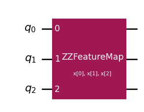
ZZ feature map

This is a particular version of the Pauli feature map that we will be able to find in Qiskit. It performs the same rotations we saw in the angle encoding but with an extra \(ZZ\) interaction between data points to capture the correlating observations to further boost their representation. We can also perform several repetitions of the mapping providing a more complex iteration.

Given that it uses \(Z\) rotations it is common to see Hadamard gates preceding those rotations so that by moving our \(|0\rangle\) states to \(|+\rangle\) will make sure those rotations have some meaningful effect.

from qiskit.circuit.library import ZZFeatureMap

feature_map = ZZFeatureMap(3)
feature_map.draw('mpl')

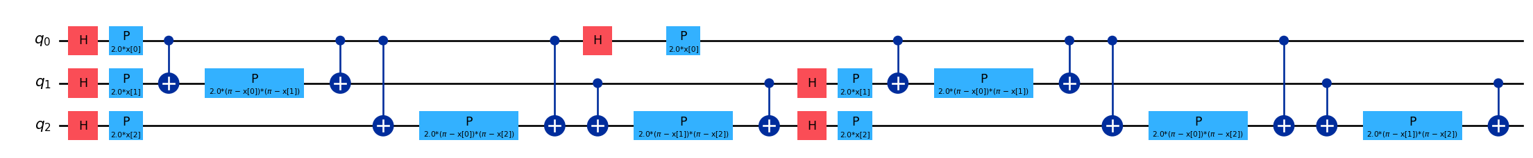
feature_map.decompose().draw('mpl', fold=-1)

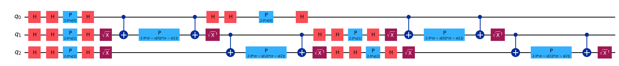
The general case allows to define a complete specification of Pauli rotations and entanglement layout so that one can customize the feature map to its specifications.

from qiskit.circuit.library import PauliFeatureMap

feature_map = PauliFeatureMap(3, paulis=["X", "YZ"], entanglement='linear')
feature_map.decompose().draw('mpl', fold=-1)

Why is this mapping good? Or bad? How many repetitions need to be used? Well, indeed, some of the approaches have no particular rational behind and are much more experimental. We can always look into the literature relevant papers exploring the qualities of each feature map trying to find the one that could be beneficial for our project (Sim, Johnson, and Aspuru-Guzik 2019).