So, now you know how a simulator works. Essentially performs the mathematical operations we expect a quantum computer will do. but there are quite some nuances on the way in which we do this. For example, it is not the same to use a simulator or an emulator.
A simulator performs specifically the actions of the mathematical framework, without any restriction or special case. Simply put, it was what the ideal machine should do. An emulator on the other hand, performs the same set of actions but considering some of the limitations a particular device could have. Essentially it is trying to show how the same actions performed by a physical machine would look like.
The of course, you have sending the job to a real device through a service like the ones offered by the IBM Quantum Platform. You will need to create an account but after that, you can submit all the circuits you want to real hardware. checkout this example.
Simulators
The actions we performed in previous exercise were mimicking the state vector of our system and performing the unitary operations that drive the state. This is often known as State Vector simulator (dah!) and it is common on some of the most used SDKs. The ability to simulate a given circuit is proportional to the resources needed to manipulate that state vector.
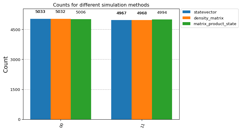
GHZ-state case
Let’s take a GHZ state as an example, a 5 qubit GHZ state.
A 5-qubit system requires a state vector in a Hilbert space of dimension \(2^5 = 32\). Each amplitude is a complex number, typically represented with double precision. So, making a back of the envelope calculation: \(32\) amplitudes \(\times\)\(16\) bytes (8 bytes real part + 8 bytes imaginary part) \(= 512\) bytes.
Beyond the state vector, a quantum simulator needs:
Quantum gates (\(H\) and \(CX\) in this case). For 5 qubits, single-qubit gates are 2×2 matrices and two-qubit gates are 4×4: ~1-2 KB per gate.
Temporary buffer for intermediate calculations of similar size.
Simulator overhead for managing the circuit, data structures and conversions: ~10-50 KB
Minimum theoretical memory: ~512 bytes + overhead ≈ 50-100 KB. Most of this goes into the simulator itself more than the simulation but as we scale those numbers up, a 10 qubit simulator manages ~16KB state vectors, 20-qubit one ~16MB and 30 qubit system uses only ~16GB just for the state vector representation. You might struggle beyond 22-25 qubits depending on how powerful your machine is.
A less common approach, given the numbers we saw before, is the usage of the Density Matrix simulator, which renders the whole evolution considering the effect of noise and the potential of obtaining a mixed-state (which in reality happens a lot but unless we work trying to emulate the work of a device, we can skip it). This not only manages a state vector but a matrix evolution on each step.
The Matrix Product State simulator is a method derived from Tensor Networks, a way to efficiently deal with large matrix operations, at least up to a precision. In many cases this method allows us to emulate larger circuits as it is the most resource efficient method although in some cases, unless you are using some bleeding-edge simulators, they do not offer the option of noise simulation.
Qiskit is not the only SDK we will be using so it is good to know this very same simulation techniques exist when, for example, using Pennylane you will have access to several devices including:
default.qubit for state vector simulation
default.mixed for dealing with mixed states
default.tensor for MPS type of simulation using QUIMB under the hood
And many more. They also include nice simulators for GPU based simulation, based on NVIDIA cuQuantum SDK via Lightning which will be really helpful when we start talking about training circuits.
If you are interested in Tensor Networks, this is not the right place, but I can recommend some resources like TensorNetwork.org to look into useful resources and some nice references to get deeper into the field (Biamonte and Bergholm 2017).
In any case, this is not a trivial task. In fact, some have already claimed to be a Herculean task (Xu et al. 2023). There is a useful guide by google on how to choose your hardware. Let’s keep it simple for now and deal with algorithm implementations.
Xu, Xiaosi, Simon Benjamin, Jinzhao Sun, Xiao Yuan, and Pan Zhang. 2023. A Herculean Task: Classical Simulation of Quantum Computers. https://arxiv.org/abs/2302.08880.